Calculate a Weighted Average in Excel & Google Sheets
SUMPRODUCT divided by SUM works in both. Google Sheets adds AVERAGE.WEIGHTED. Full setup, worked examples, error fixes and a live practice sheet.
excelgoogle sheetsformula
SUMPRODUCT divided by SUM works in both. Google Sheets adds AVERAGE.WEIGHTED. Full setup, worked examples, error fixes and a live practice sheet.
excelgoogle sheetsformula
A support team reports customer satisfaction of 4.14 out of 5. The real figure is 4.44. The
spreadsheet used =AVERAGE() across five channel scores and never looked at the ticket counts beside
them.
That 0.30 gap is one function call wide. Excel has no weighted average function, so you build it from SUMPRODUCT and SUM. Google Sheets hands you AVERAGE.WEIGHTED instead, and that convenience has a catch worth knowing before you send the file anywhere.
This guide covers the setup, both platforms, percentage and numerical weights, every error code you will meet, and a live sheet you can type into. The weighted average calculator and the weighted mean calculator will check your work, and how to calculate a weighted average covers the arithmetic behind the formulas.
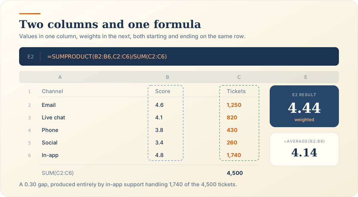
Put the values in one column and the weights in the next, with each pair on the same row. Both ranges must start and end on the same row. Every formula on this page depends on that alignment and nothing else.
Column B holds what you measured. Satisfaction scores, prices, grades, returns. One number per row, formatted as a number rather than text.
Column C holds how much each row counts. Ticket volumes here, but units, credits or dollars work identically. Never mix weight types in one column.
Each row is one pair. Sorting column B without column C destroys the relationship, which is why you sort the whole table or nothing at all.
=SUMPRODUCT(B2:B6,C2:C6)/SUM(C2:C6) Returns 4.44
=SUMPRODUCT(B2:B6,C3:C7)/SUM(C3:C7) Returns 3.83, silently
B2:B6 and C2:C6 both cover five rows. B2:B6 against C3:C7 also covers five rows, which is exactly why the mistake survives. No error appears and the number looks fine.
Use =SUMPRODUCT(B2:B6,C2:C6)/SUM(C2:C6). SUMPRODUCT multiplies each value by its weight and adds
the products. SUM totals the weights. Excel has no built-in weighted average function, so this pair
is the standard approach.
Two functions, one cell, no helper column. SUMPRODUCT builds the numerator and SUM builds the denominator. Microsoft documents SUMPRODUCT as an array multiplier, and weighted averages are its most common real use.
=SUMPRODUCT(B2:B6,C2:C6)/SUM(C2:C6) Works unchanged in Excel 2007 through Microsoft 365, Excel for the web, and Google Sheets.
SUMPRODUCT pairs the ranges row by row. Row 2 gives 4.6 times 1,250, which is 5,750.
It then adds every product without you asking. Five rows collapse into 19,982 inside a single function call.
SUM returns 4,500 and the slash does the rest. That division is what converts a weighted sum back onto the original scale.
Five support channels scoring 4.6, 4.1, 3.8, 3.4 and 4.8 across 1,250, 820, 430, 260 and 1,740 tickets give a weighted sum of 19,982 and a total weight of 4,500, producing a satisfaction score of 4.44.
| Channel | Score | Tickets | Score × tickets |
|---|---|---|---|
| 4.6 | 1,250 | 5,750 | |
| Live chat | 4.1 | 820 | 3,362 |
| Phone | 3.8 | 430 | 1,634 |
| Social | 3.4 | 260 | 884 |
| In-app | 4.8 | 1,740 | 8,352 |
| Totals | — | 4,500 | 19,982 |
Click an empty cell, type the formula, press Enter. Select the ranges with the mouse rather than typing them, because a dragged selection cannot land on the wrong starting row.
Put =SUM(C2:C6) in its own cell even though the main formula already contains it. Seeing 4,500 on
screen is how you catch a missing row before it reaches a report.
The plain AVERAGE of column B returns 4.14. Ticket volume pulls the real satisfaction score to 4.44, because in-app support handles 1,740 of the 4,500 tickets.
19,982 ÷ 4,500 = 4.44
Set every ticket count to zero in the sheet above and the cell returns #DIV/0!. That is the formula
telling you the truth, not failing.
Google Sheets offers =AVERAGE.WEIGHTED(B2:B6,C2:C6), a dedicated function that handles the
division internally. It also accepts the SUMPRODUCT formula, which returns the identical result and
survives an export to Excel.
One function, two ranges, done. Google documents AVERAGE.WEIGHTED as finding the weighted average of a set of values given their weights, which is exactly what it does.
=AVERAGE.WEIGHTED(B2:B6,C2:C6) Values first, weights second. Reversing the arguments returns a number, and a wrong one.
The Excel formula works here without modification. Sheets implements SUMPRODUCT identically, so teams that move files between applications standardise on it.
=SUMPRODUCT(B2:B6,C2:C6)/SUM(C2:C6) The only built-in route. Excel has no dedicated weighted average function.
=SUMPRODUCT(B2:B6,C2:C6)/100 Shortcut when the weights are percentages that already total 100.
Works in Excel 2007 through Microsoft 365, and in Excel for the web. No dynamic arrays required.
=AVERAGE.WEIGHTED(B2:B6,C2:C6) Purpose-built, shorter, and it handles the division for you.
=SUMPRODUCT(B2:B6,C2:C6)/SUM(C2:C6) Identical result, and the version that survives an export to Excel.
AVERAGE.WEIGHTED is a Google Sheets function. Export the file to .xlsx and it breaks.
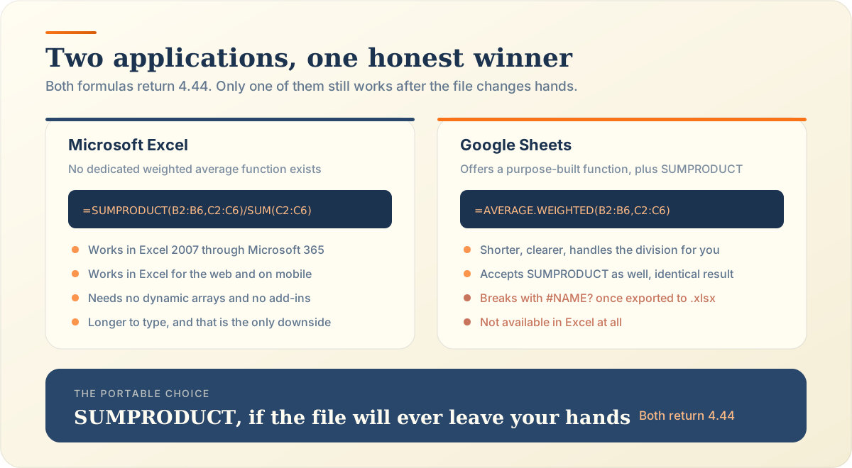
Enter the same five channels and ticket counts, then apply AVERAGE.WEIGHTED to columns B and C. It returns 4.44, matching the SUMPRODUCT formula to every decimal place.
Scores in B2:B6, ticket counts in C2:C6, headers in row 1. Identical layout to the Excel version, because the layout is the part that never changes.
Type =AVERAGE.WEIGHTED(B2:B6,C2:C6) and press Enter. Sheets returns 4.44 with no division step
anywhere in the formula.
Put =SUMPRODUCT(B2:B6,C2:C6)/SUM(C2:C6) in the cell below it. Same 4.44, arrived at the long way.
Two cells showing the same number is the cheapest verification available. If they disagree, one formula is pointing at the wrong range, and a glance at each tells you which.
Percentage weights work exactly like any other weights. Enter them as whole numbers or decimals, keep the notation consistent down the column, and use the same SUMPRODUCT formula. Dividing by SUM handles either scale automatically.
Type 35 or 0.35, but never both in one column. A survey weighted 35, 20, 15 and 30 percent across scores of 8.2, 7.4, 6.9 and 8.8 returns 8.03.
Identical entry, identical formula. Cell formatting as a percentage changes the display only, so a cell showing 35% holds 0.35 underneath and the formula reads that.
You rarely need to. Dividing by the total weight rescales any column, which is the whole argument for never hard-coding the denominator. The weighted percentage calculator shows each row’s share while you work.
SUM returns 100 and the formula divides by 100. You could hard-code that, but the moment somebody adds a fifth row your fixed denominator quietly becomes wrong.
Nothing changes. SUM(C2:C6) returns whatever the weights actually total, and the division adjusts
for it. Weights of 4,500 tickets, 70 percentage points or 130 rubric points all work with the same
formula.
Always reference the range, never a typed number. SUM(C2:C6) stays correct when the data changes,
and /100 does not.
Our ticket counts total 4,500 and nothing about the formula noticed. This is the ordinary case in business data, as what a weighted average is explains across other fields.
Three of the four survey categories cover 70 points. The weighted sum of 538.5 divided by 70 gives 7.69, a valid partial result rather than a broken one.
A rubric scoring out of 40, 35, 30 and 25 totals 130. The weighted sum of 1,014 divided by 130 returns 7.80, and no conversion step was required anywhere.
SUMPRODUCT removes the need for a helper column entirely. It performs the row-by-row multiplication inside the function, so one cell replaces a whole column of value times weight calculations.
Before SUMPRODUCT, people built a column D of =B2*C2 formulas and summed it. One function does that
work invisibly.
Fewer cells mean fewer places to break. A helper column can be sorted, filtered or deleted by someone who did not realise it fed a formula.
When you need to see the contributions. Auditing a disputed grade or invoice is far easier with each row’s product visible, which is why the weighted grade calculator shows them rather than hiding them.
Four formulas cover almost every case: basic SUMPRODUCT, the Sheets-only AVERAGE.WEIGHTED, a whole-column version for growing data, and a conditional version that filters rows before averaging.
=SUMPRODUCT(B2:B6,C2:C6)/SUM(C2:C6) The default. Use it unless you have a specific reason not to.
=AVERAGE.WEIGHTED(B2:B6,C2:C6) Shorter and clearer, but it returns #NAME? the moment the file opens in Excel.
=SUMPRODUCT(B2:B1000,C2:C1000)/SUM(C2:C1000) Blank rows contribute zero to both halves, so new data is picked up without editing the formula.
=SUMPRODUCT((A2:A100="Email")*B2:B100*C2:C100)/SUMIF(A2:A100,"Email",C2:C100) The comparison produces TRUE and FALSE, which multiply as 1 and 0, so non-matching rows drop out.
Six problems account for nearly every broken weighted average: mismatched range sizes, misaligned pairs, the wrong denominator, using AVERAGE by mistake, a zero total weight, and text sitting in a numeric range.
Put =SUM(C2:C6) in an empty cell. If it returns 0, this is your answer.Compare =ROWS(B2:B6) against =ROWS(C2:C6). They must match exactly.Start typing the function name. If no autocomplete appears, it is not available here.Compare the total weight against what you expected. Then check row 2 by hand.Excel returns #VALUE! immediately. Compare =ROWS(B2:B6) against =ROWS(C2:C6) and resize
whichever range is short.
The dangerous one. Offset ranges return 3.83 instead of 4.44 with no warning at all, because five rows paired with five rows is still valid arithmetic.
Hard-coding /100 when the weights total 4,500 inflates the answer beyond recognition. Reference
SUM() and the problem cannot occur.
This is the error that produced our opening 4.14. It throws nothing, reads plausibly, and ignores an entire column of data. The difference between the two methods is covered in weighted average vs simple average.
#DIV/0! means SUM() returned zero. Usually the weights are stored as text, which sums to nothing
while still looking like numbers on screen.
Left-aligned numbers are text. Run the column through Data then Text to Columns in Excel, or multiply by 1 in a scratch cell to confirm.
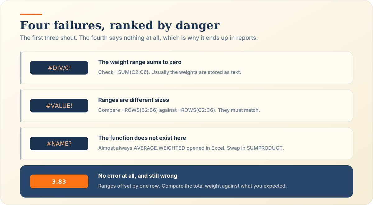
Check the total weight against what you expected, confirm the weighted sum separately, recompute one row by hand, and compare the answer against the simple average. Four checks, well under two minutes.
Put =SUM(C2:C6) in a visible cell. Our 4,500 tickets should match the support system’s own count,
and a gap means a row is missing.
Put =SUMPRODUCT(B2:B6,C2:C6) in another cell. Seeing 19,982 on its own makes the two halves of the
calculation independently auditable.
Take row 2 alone. 4.6 times 1,250 is 5,750, and that figure should appear if you compute it in a scratch cell. One row proves the pairing.
Add =AVERAGE(B2:B6). It returns 4.14, and the gap of 0.30 is the value your weighting is adding.
Identical results mean your weights are all equal or something is wrong.
Excel requires SUMPRODUCT divided by SUM. Google Sheets offers AVERAGE.WEIGHTED as well. Both produce identical results, but only SUMPRODUCT survives moving a file between the two applications.
Longer to type and completely dependable. It has worked the same way since Excel 2007 and needs no dynamic arrays, no add-ins and no subscription tier.
Shorter, clearer to a colleague reading your sheet, and locked to one platform. That trade is fine for a file that will never leave Google Drive.
One formula, two applications, zero translation. Every finance team I would trust with a shared model standardises on this for exactly that reason.
SUMPRODUCT, without argument. If there is any chance the file gets downloaded as .xlsx, emailed or opened by someone on a different platform, use it and accept the extra typing.
Use =SUMPRODUCT(B2:B6,C2:C6)/SUM(C2:C6), with values in the first range and weights in the second.
SUMPRODUCT multiplies each pair and adds the products, while SUM totals the weights for the
denominator. Both ranges must be the same size and start on the same row. The formula works in every
version of Excel from 2007 onward, including Excel for the web.
No, and it never has. There is no WEIGHTEDAVERAGE, AVERAGE.WEIGHTED or similar function in any
version of Excel, including Microsoft 365. SUMPRODUCT divided by SUM is the accepted approach and
appears throughout Microsoft’s own documentation and templates. If you typed a weighted average
function and got #NAME?, you were using a Google Sheets formula by mistake.
It is a purpose-built function that takes values and weights and returns the weighted average
directly. The syntax is =AVERAGE.WEIGHTED(values, weights), so
=AVERAGE.WEIGHTED(B2:B6,C2:C6) returns 4.44 on our data. It handles the division internally, which
makes formulas shorter and easier for colleagues to read. It exists only in Google Sheets.
Yes, and often you should. Google Sheets implements SUMPRODUCT identically to Excel, so
=SUMPRODUCT(B2:B6,C2:C6)/SUM(C2:C6) returns the same 4.44 as AVERAGE.WEIGHTED. The advantage is
portability. A sheet built on SUMPRODUCT keeps working after someone downloads it as .xlsx, while
AVERAGE.WEIGHTED breaks with #NAME?.
No. Weights can total 4,500 tickets, 70 percentage points, 130 rubric points or any positive number.
Dividing by SUM() rescales whatever you used into proportions automatically. Percentages totalling
100 are convenient, nothing more. The one total that fails is zero, which produces #DIV/0! because
nothing can be divided by it.
#VALUE! almost always means the two ranges are different sizes, so check =ROWS() on each.
#DIV/0! means the weights sum to zero, usually because they are stored as text rather than numbers.
#NAME? means the function does not exist in your application. If no error appears but the number
looks wrong, your ranges are probably offset by a row.
Because the weights are doing their job. =AVERAGE(B2:B6) gives every score one equal vote, so a
channel handling 260 tickets counts as much as one handling 1,740. That is why our data returns 4.14
unweighted and 4.44 weighted. The two match only when every weight is identical, which makes an
equal-weight test a useful sanity check.
Yes, and SUMPRODUCT exists precisely for this. It performs the row-by-row multiplication internally,
so a single cell replaces an entire column of =B2*C2 formulas. Helper columns remain useful when
you need to show each row’s contribution for an audit, such as a disputed grade or a contested
invoice. For everything else, one cell is safer and tidier.
Every tool below runs the same arithmetic as these formulas and prints the weighted sum beside the total weight, which makes checking a spreadsheet straightforward.
That support team now reports 4.44 and reconciles against their ticket system. The fix was one formula and a column that had been sitting there all along. If your data is academic rather than operational, calculating weighted grades and GPA covers the same mechanics with credit hours. More questions about weighting are answered case by case, and the weighted average calculator prints every intermediate figure so you can match it against your sheet cell by cell. Which formula is in your file right now?
Divide by whatever the weights actually total, not by 100. Worked examples above and below 100, normalising, and when a wrong total is a real warning.
weightsnormalizationweighted average
Multiply each holding's return by its share of portfolio value, then add. Formula, worked example, contributions, asset classes and the measures it is not.
portfolioinvestment returnsweighted average
Calculate Weighted Average Online
The weighted average calculator multiplies each value by its weight, adds the weighted sum, divides by the total of weights, and prints the weighted average beside the standard arithmetic mean. Course grades, GPA, portfolio returns, and probability distributions all run through the same 4 steps.
Open the Weighted Average Calculator