How to Check and Fix Weighted Average Calculation Errors
Most weighted average errors pass a range check. How to audit values, weights, products and totals, fix the mistake, and prove the corrected result.
errorstroubleshootingweighted average
Most weighted average errors pass a range check. How to audit values, weights, products and totals, fix the mistake, and prove the corrected result.
errorstroubleshootingweighted average
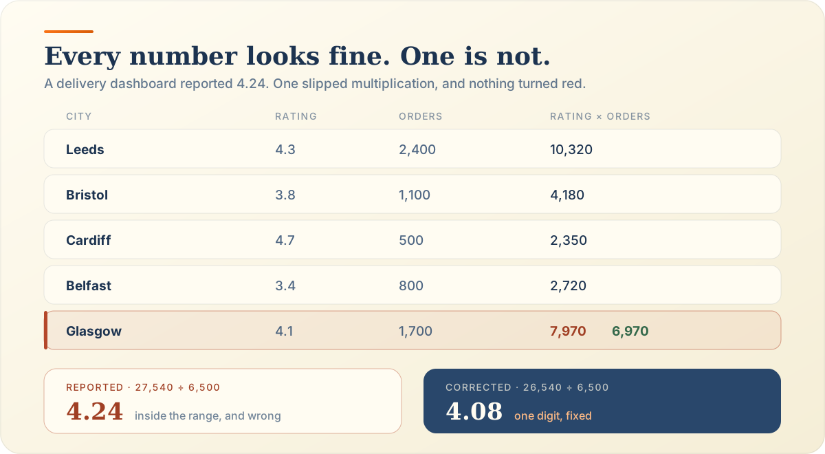
A delivery app’s dashboard reported an average rating of 4.24 across five cities. The real figure was 4.08. One product in the spreadsheet read 7,970 where 4.1 × 1,700 is 6,970.
Nothing turned red. The number sat comfortably inside the 3.4 to 4.7 range of the ratings, so the usual sanity check waved it through. That is the uncomfortable truth about weighted average errors: the obvious ones get caught, and the believable ones get published.
This guide shows how to check a weighted average at each stage, fix what you find, and prove the correction. The weighted average calculator and the weighted mean calculator print every intermediate total, and how to calculate a weighted average covers the method itself.
It is any fault in the values, weights, products, total weight or final division. Each stage has its own typical errors, so checking stage by stage finds them faster than staring at the result.
A rating typed as 3.4 instead of 4.3. Transposed digits are the classic culprit.
An extra zero turns 500 orders into 5,000 and pulls the answer toward that row.
A slipped multiplication, like our 7,970. The inputs are right and the arithmetic is not.
A row left out of the sum, or a duplicated one. The denominator then describes different data.
Dividing by 100 or by the number of rows instead of by the total weight.
Verify the values, verify the weights, recompute each product, confirm the total weight against its source, then redo the division. Work in the order the calculation runs.
Pass. All five ratings match the app export.
Pass. 2,400 + 1,100 + 500 + 800 + 1,700 = 6,500.
Pass, and that is the trap. 4.24 sits comfortably inside 3.4 to 4.7.
Fail. Glasgow shows 7,970, but 4.1 × 1,700 is 6,970.
Fail. The reported 4.24 cannot be reproduced. Corrected, 26,540 ÷ 6,500 = 4.08.
Compare every value with its source export, not with your memory of it.
Check each weight against the ledger it came from. Our order counts come from the delivery system.
Recompute every value × weight independently. This is the check that caught 7,970.
2,400 + 1,100 + 500 + 800 + 1,700 = 6,500, matching the ledger exactly.
Divide the corrected weighted sum by the verified total: 26,540 ÷ 6,500 = 4.08.
The formula is the sum of each value times its weight, divided by the sum of the weights. Check the numerator and the denominator separately, then confirm every value sits beside its own weight.
Weighted average = ∑(value × weight) ÷ ∑ weight
It should be large. A weighted sum of 26,540 for ratings near 4 is normal, because it has not been divided yet.
It must be the sum of the weights, never the row count and never an assumed 100.
Read each row left to right. Leeds carries 2,400 orders, and nothing else.
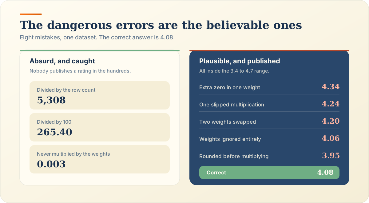
Seven errors cause most wrong answers. Three produce absurd results that readers catch. The other four produce believable numbers inside the range of the data, which is why they survive.
26,540 ÷ 5 gives 5,308. Absurd, and mercifully obvious.
26,540 ÷ 100 gives 265.40. The weights total 6,500, not 100, as weights that do not total 100% explains.
Dividing the plain sum of ratings by 6,500 gives 0.003. The weighted sum was never built.
Same fault, different spreadsheet. The numerator holds raw values while the denominator holds weights.
Swapping the Leeds and Cardiff weights gives 4.20. The total still reads 6,500, so only a row-by-row check finds it.
The plain average is 4.06. Close enough to look right, and it ignores every order count.
Rounding ratings to whole numbers before weighting gives 3.95. Round once, at the end.
Name what each weight represents, find any missing or duplicated rows, put every weight in one unit, and replace weights that do not describe the data. Then recalculate from scratch.
“Orders delivered per city.” If you cannot finish that sentence, see how to choose the right weights.
A blank weight contributes nothing to either total. Confirm the row is meant to be excluded.
A city listed twice inflates both totals. Compare the row count with the source.
Orders in thousands beside orders in units makes one row a thousand times too heavy.
Cardiff’s 500 orders typed as 5,000 give 4.34 and a total weight of 11,000. The ledger says 6,500, which exposes it immediately.
Decide whether the weights are supposed to describe a complete allocation. If they are, find the missing category. If they are not, divide by their actual total and the problem disappears.
Syllabus and portfolio weights should. Order counts, credits and units should not.
Add the column and write the figure down. Our weights total 6,500.
Divide each weight by the total. Leeds becomes 2,400 ÷ 6,500, or 36.9%.
26,540 ÷ 6,500 = 4.08, with or without normalizing first.
Normalized weights must sum to exactly 1, or 100%. Anything else means a divisor went wrong.
Confirm each value sits beside its own weight, in the same order as the source, with no shifted or missing rows. Equal row counts are necessary but do not prove the pairs are right.
Glasgow’s 4.1 belongs with Glasgow’s 1,700 orders. Check the label, not just the position.
Sorting one column without the other scrambles every pair silently.
A one-row shift pairs every value with its neighbour’s weight and produces a plausible answer.
Five values need five weights. A mismatch in a spreadsheet usually returns an error, which is a favour.
Recompute every value × weight, add the products again in a different order, and compare with the original sum. A difference points straight at the faulty row.
4.3 × 2,400 = 10,320. 4.1 × 1,700 = 6,970. Do every row, not just the suspicious ones.
10,320 + 4,180 + 2,350 + 2,720 + 6,970 = 26,540.
The report used 27,540. A gap of exactly 1,000 points at a single mistyped digit.
Round-number gaps like 1,000, 100 or 10 almost always mean one slipped digit in one product.
Divide the weighted sum by the total weight, confirm the result sits between the smallest and largest value, compare it with the simple average, and recalculate by a second method.
26,540 ÷ 6,500 = 4.08
A result outside 3.4 to 4.7 is impossible. A result inside proves very little.
4.08 sits just above 4.06, because Leeds, the busiest city, rates 4.3. A large gap needs an explanation.
Normalize the weights and add weight share × value. Two methods agreeing is strong evidence.
Every field has a signature error. Grades lose a category, prices lose a quantity, portfolios mix dates, inventory forgets opening stock, frequencies drop a bucket, and business metrics mix units.
Check that syllabus weights total 100 and credits match the transcript. The weighted grade calculator flags a shortfall, and weighted grades and GPA covers credit hours.
Confirm quantities, not purchase counts, are the weights.
Check every return covers the same period, as weighted portfolio returns explains.
Confirm beginning inventory is in both totals. The weighted average cost calculator includes it by default.
Check the frequencies sum to the number of observations you actually have.
Confirm every weight uses one unit and one period.
Check both ranges start and end on the same rows, confirm the SUMPRODUCT and SUM ranges match, and compare the spreadsheet result with a hand calculation of one row.
B2:B6 must cover exactly the five ratings, no header, no blank.
C2:C6 must start on the same row as the values.
=SUMPRODUCT(B2:B6,C2:C6) should return 26,540 on its own.
=SUM(C2:C6) should return 6,500, matching the ledger.
Multiply one row by hand. If B2 × C2 is not 10,320, the ranges are wrong. The full setup is in the Excel and Google Sheets guide.
Correct the cell references, realign the ranges, reference SUM instead of typing a total, clean blank or text cells, and guard against a zero total weight.
Click the formula and check the highlighted ranges on the grid. They should frame the same rows.
Change C3:C7 back to C2:C6. Offset ranges return a believable number, never an error.
Replace a typed 100 with SUM(C2:C6), so the total updates with the data.
Left-aligned numbers are text, and SUMPRODUCT treats them as zero. Microsoft documents this in the SUMPRODUCT reference.
#DIV/0! means the weights sum to zero. Wrap the formula in IFERROR only after you know why.
Check the ranges, confirm AVERAGE.WEIGHTED lists values before weights, cross-check with SUMPRODUCT and SUM, clean invalid cells, and compare the final figure with a manual calculation.
Both must cover the same rows, starting at the same row.
Values come first, weights second. Google’s AVERAGE.WEIGHTED reference confirms the order. Reversed arguments return a number, and a wrong one.
Put =SUMPRODUCT(B2:B6,C2:C6)/SUM(C2:C6) beside it. Both should read 4.08.
Remove stray text and currency symbols typed as characters.
Two formulas agreeing, plus one row checked by hand, is enough.
Confirm the result sits inside the range, find the heaviest weights, check which values contribute most, and explain any large gap from the simple average before trusting it.
The correct weighted average for this data is 4.08. The ratings run from 3.4 to 4.7, and the simple average is 4.06.
Inside the range is required. It is not proof.
Leeds holds 2,400 of 6,500 orders, or 36.9%. The answer should lean toward its 4.3.
Leeds contributes 10,320 of 26,540. If the largest contributor looks wrong, everything does.
The weighted 4.08 sits 0.02 above the simple 4.06. The broken 4.24 sat 0.18 above it, with no heavy high-rated city to explain the jump.
A result near the minimum or maximum means one row dominates. Confirm that is real before reporting it.
A dashboard reported 4.24. Values and weights checked out, but the Glasgow product read 7,970 instead of 6,970. Correcting it gives a weighted sum of 26,540 and an average of 4.08.
The reported average is 4.24. Every number above looks plausible, which is exactly why the error survived.
The reported 4.24 could not be reproduced from the source data.
All five ratings and all five order counts match their sources. The inputs are fine.
Recomputing each product exposes Glasgow: 4.1 × 1,700 is 6,970, not 7,970.
| City | Rating | Orders | Rating × orders |
|---|---|---|---|
| Leeds | 4.3 | 2,400 | 10,320 |
| Bristol | 3.8 | 1,100 | 4,180 |
| Cardiff | 4.7 | 500 | 2,350 |
| Belfast | 3.4 | 800 | 2,720 |
| Glasgow | 4.1 | 1,700 | 6,970 |
| Totals | — | 6,500 | 26,540 |
26,540 ÷ 6,500 = 4.08.
4.08 sits inside the range, slightly above the simple average, and a spreadsheet returns the same figure.
Seven checks in calculation order catch almost every error. Run them all, because the range check that comes last is the one most likely to pass a wrong answer.
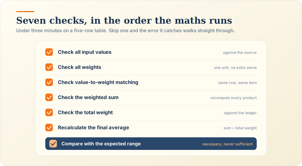
Against the source, one by one.
One unit, no extra zeros, no blanks.
Same row, same item.
Recompute every product.
Against the ledger or syllabus.
Weighted sum ÷ total weight.
Inside the range, and leaning toward the heaviest weights.
Usually one of five faults: a wrong value, a wrong weight, a slipped product, a wrong total weight, or division by the wrong number. Check each stage in order rather than guessing from the final figure.
Verify the values and weights against their sources, recompute each product, confirm the total weight, then redo the division. A second method, such as normalized weights, confirms the result.
Dividing by the number of values or by 100 instead of the total weight. Those are easy to spot. The most damaging are slipped products and swapped weights, because they produce believable results.
Because that converts each weight into its share of the whole. Any other divisor gives a number that describes nothing, like 265.40 for a rating out of 5.
Nothing, if you divide by their actual total. Our weights total 6,500 and give a correct 4.08.
No. With non-negative weights it always lands between the smallest and largest value. A result outside that range proves an error.
Either every weight is equal, or the weights never entered the formula. Check that the weight column is actually referenced.
Check whether the expectation came from a simple average. Otherwise, recompute the products and the total weight, because those hide most believable errors.
Put =SUMPRODUCT(B2:B6,C2:C6) and =SUM(C2:C6) in separate cells, check both against a manual
calculation, and confirm the ranges start on the same row.
Align both ranges to the same rows, divide by SUM() of the weight range, and convert any text cells
to numbers. The
weighted percentage calculator gives an independent check.
Multiply each value by its weight, add the products, add the weights, and divide. Then compare with the simple average and explain the gap.
Reference totals instead of typing them, keep values and weights in adjacent columns, never sort one without the other, and run the seven-point checklist before sharing any result.
Back to that dashboard. The fix took one digit, and finding it took one check nobody had run: recomputing each product. Run the checks in order, and do not stop at the range check. More questions about weighting are answered case by case, and the weighted average calculator prints each product so a slipped digit has nowhere to hide. Which check does your team skip?
Divide by whatever the weights actually total, not by 100. Worked examples above and below 100, normalising, and when a wrong total is a real warning.
weightsnormalizationweighted average
Multiply each holding's return by its share of portfolio value, then add. Formula, worked example, contributions, asset classes and the measures it is not.
portfolioinvestment returnsweighted average
Calculate Weighted Average Online
The weighted average calculator multiplies each value by its weight, adds the weighted sum, divides by the total of weights, and prints the weighted average beside the standard arithmetic mean. Course grades, GPA, portfolio returns, and probability distributions all run through the same 4 steps.
Open the Weighted Average Calculator